Introduction
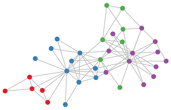
The latest fad in deep learning circles has been the graph neural network (or GNN), a deep learning model that takes in graph structures and learns on its attributes, whether it be nodes, edges, or even entire graphs. However, despite advancements in the field regarding attention and transformers, many graph networks still struggle to learn over longer distances, defeating the purpose of many tasks that graph structures encode. Our project aims to benchmark certain networks’ performances on these long range tasks, introduce our own long range benchmark dataset, and use techniques on both the dataset and network to determine which are best for long range performance.
Our website’s main purpose is to visualize our datasets and our results, if you want to see more theoretical portions of our project (such as the math behind models and optimization techniques), please refer to our report.
Methodology
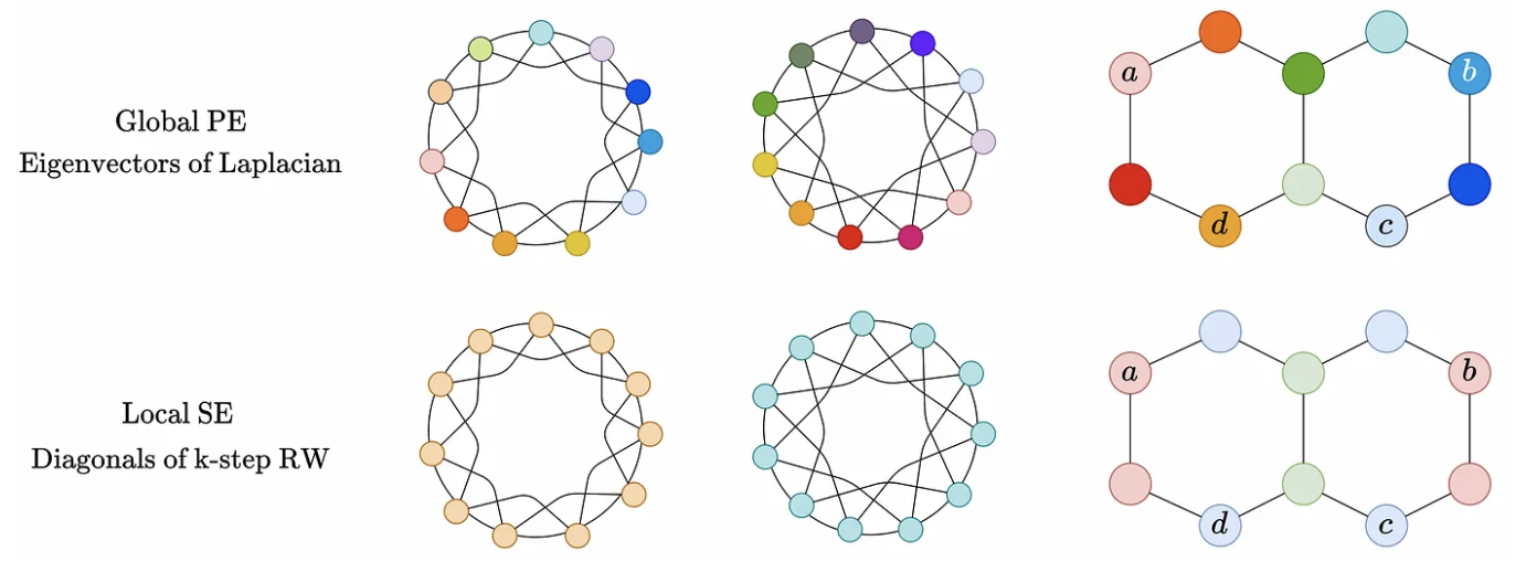
For this project, we trained 5 different graph neural networks on 3 datasets and optimized each dataset/model differently to see which combination would run best. We manipulated data by randomly adding edges throughout the dataset’s nodes to decrease average node distances, and added positional encodings given either by laplacian eigenvectors (LapPE) or by a random walk matrix (RWSE). We also added partial attention to certain models that supported it.
For an extended methodology, refer to the report.
| Datasets | Model Types | Optimization Technique |
|---|---|---|
|
|
|
Datasets
Our models were benchmarked, and performance recorded, on 3 different datasets with 2 different tasks.
PascalSP-VOC (Node)
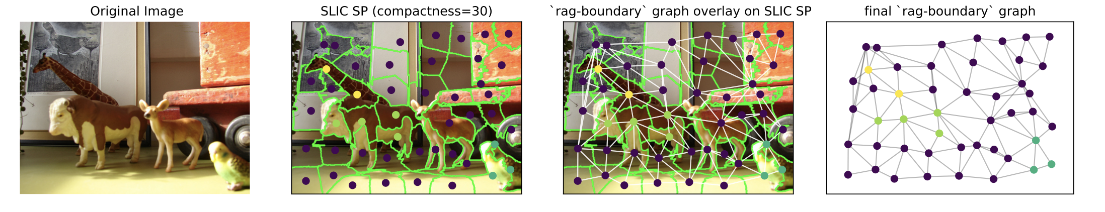
Based on the Pascal-VOC 2011 dataset, each image is passed through the SLIC algorithm to create superpixels, which are each categorized into one of the 21 classes in the original segmentation (20 classes of items, plus 1 for no category). The goal of this task is to predict the class of a superpixel region based on 14 node features (12 RGB values, 2-dim point in space representing center-of-mass for superpixel) and 2 edge features (average value of pixels across boundary, count of pixels on boundary).
Created and sourced from the Long Range Graph Benchmark.
Peptides-Functional (Graph)
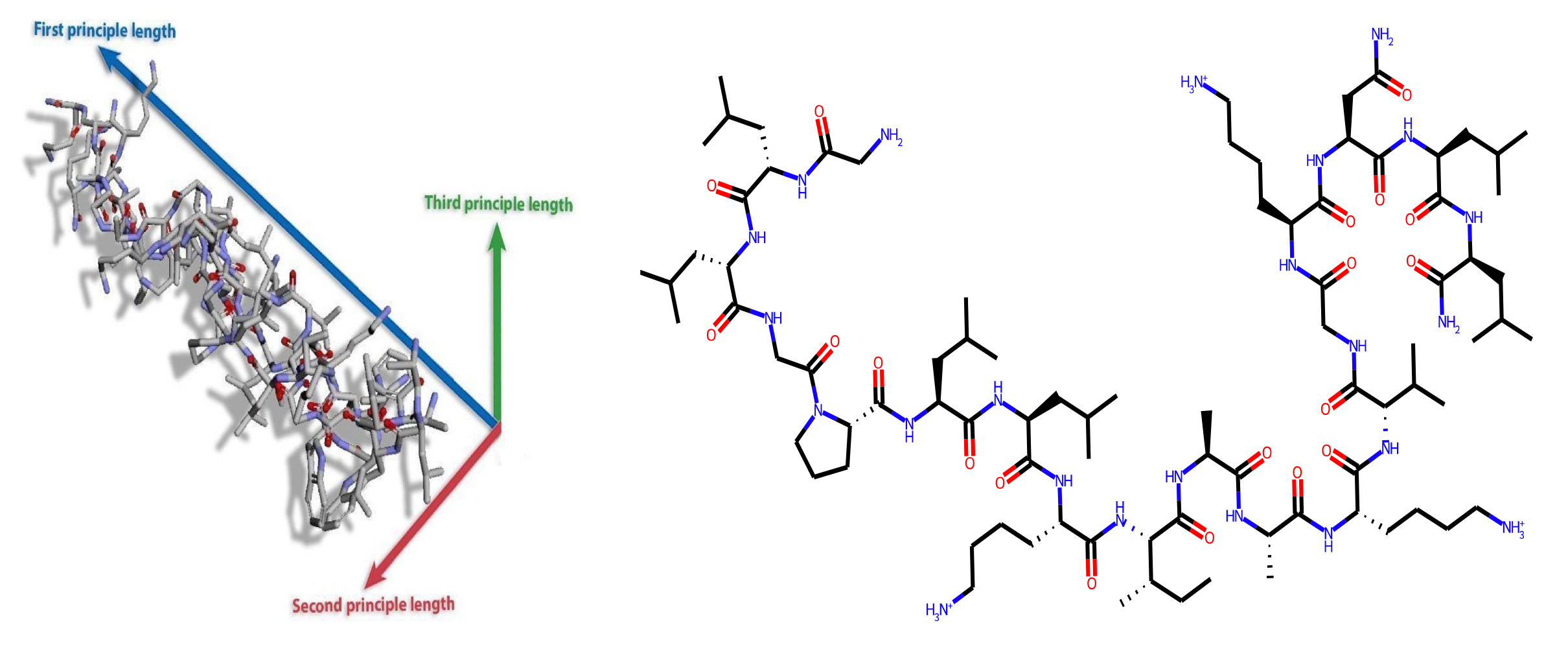
Based on the SATPdb dataset, 15,535 peptides were converted to graphs through molecular SMILES, with edge and node features coming from the Open Graph Benchmark feature extraction. Nodes are created from non-hydrogen atoms and edges are created from the bonds between these atoms. It should be noted that multi dimensional positional data for these molecules is not encoded into these graphs whatsoever, and instead graphs prioritize 1D amino acid chains, meaning that the network needs to learn its own positions for this dataset.
Created and sourced from the Long Range Graph Benchmark.
Princeton Shape Benchmark (Graph)
The Princeton Shape Benchmark is a 3D object dataset, in which a model must learn to classify 3D objects based on their shape into one of many categories. To form these 3D files as graphs, we used a k nearest neighbor method to create edges between the closest n neighbors of any node, and stored its position as features for each node to create a positional encoding.
For this project, we used the “coarse-2” class split, which splits the 3D objects into 7 different classes. Each object in each class can either be the entire object (i.e. a car, a human) or partial components of something in that class (i.e. a wheel, a leaf).
Class 1: Vehicles
All types of vehicles made it into this dataset, as well as many common vehicle components. All the vehicle data was very clear, with good mesh connections and high quality polygons for even the most complex shapes. There was also an extremely diverse pool of data, which included motorcycles, boats, and helicopters. Components of common vehicles, such as wheels, steering wheels, and more, were also included in the class. With all of this in mind, the vehicle class was one of the most cleaned classes in the entire dataset and we felt would be one of the easier classes to predict, since there are clearer patterns in vehicle shapes.
Class 2: Animal
The animal class had plenty of variety that included land, sea, and air animals. The sheer number of different animals, including bugs, humans, housepets, fish, and birds meant that animals was one of the biggest classes of the dataset. However, unlike the previous vehicles class, the model could have a hard time predicting on an animal that it did not see before in the dataset, rendering this class much harder to predict compared to a common vehicle (such as a car).
Despite these shortcomings, the shapes in the class were well cleaned and intuitive for a human to classify.
Class 3: Household
This was one of the most confusing classes of the dataset. The shapes above are intuitively “household” objects, but the object below?
This sword, along with a fencing sword, a bottle, and even a hat made it into the “household” class. We infer that the “household” class can refer to both components of the actual house, as well as the household items that can be found in an everyday home, but this creates a much more broad category than the name implies. Almost anything in the household class can be put into another class, such as the furniture class or the miscellaneous class. Even portions of the household can be classified as “building” items, which would defeat the purpose of seperately classifying building features and entire buildings.
Besides the misclassifications of this class, most objects seem to be clean and neatly meshed, meaning that a less coarse classification (maybe coarse-1, or base) would most likely capture the entirety of this class. For the purposes of this project, we kept this class intact.
Class 4: Building
The building class is extremely simple and most objects recognizable by humans as everyday buildings. The structure of many resembled typical houses, and went so far as futuristic skyscrapers with multiple ladder-like rungs hanging off the walls. In terms of classification, we thought that the class itself would be a pretty easy one to spot patterns in.
However, some polygons and meshes in this class were messy and ultimately blurred the final product (see the first object displayed). This could have an impact on the graph created by the model, and ultimately leave our algorithm confused with strange polygons and angles in the mesh.
Class 5: Furniture
The furniture class includes some more basic household objects and furniture, all of which is well cleaned and easily recognizable.
Class 6: Plant
The plant class goes from household potted plants to full grown trees, all of which have very clean geometry. There were also parts of plants, such as leaves and stems. In general, the plants are all easily recognizable and their models are cleaned well.
Class 7: Miscellaneous
This class includes a variety of different models, most of which could go into their own class. Among the models were a lot of faces and silhouettes, as well as multiple countries modelled in 3D. The models in this class were cleaned well, but the diversity of objects means that this class would be extremely hard to consistently predict correctly.
Results and Findings
Detailed tables of results can be found in the appendix:
For all datasets, the best model was SAN, with either LapPE or RWSE applied and occasionally edges added.
-
Most models, except for PSB, performed best without the added edges. That means that, in order for the models to learn and generalize well on ALL data (not just training data), adding edges is unnecessary and even harmful to the overall accuracy of the model. PSB edges were added through k nearest neighbors, so it is possible by doubling them (from 3 to 6) we were still underfitting the edge count for 3D shapes.
-
SAN trained faster than previously cited (LRGB, GraphGPS), most likely due to advancements in GPU hardware. Training time was brought down from 60 hours in previous benchmarks to 2-3 hours in our benchmark, while keeping metrics the same if not higher.
-
Laplacian encoding and Random Walk encoding take up time at the beginning of training, since the model needs to calculate laplacian matrices and eigenvalues before the training begins. This takes up more time the larger the dataset is, and took the longest on our PSB dataset.
-
All models benefitted heavily from a transformer based model, more than just encoding or edge adding could do. PSB saw the biggest improvement just from GCN to SAN.
-
Partial with distance weighting seemed to hurt our results in all datasets, and edges/encodings needed to be added for distance weighting to become viable. Distance weighting did not work at all on Pascal.
-
Edge adding techniques did not individually improve model performance, but combining edge adding with other encoding techniques or transformers improved model performance compared to adding encoding or transformers separately.
Visualizations
Select a dataset, model, techniques, and metric to visualize!
Conclusion
In conclusion, we have explored the effectiveness of various transformer-based approaches in improving the performance of graph neural networks. Our findings suggest that incorporating transformer-based approaches can lead to more efficient and scalable GNN models that can effectively capture long-range interactions in larger graphs. Our result shows that the addition of partial graph attention can significantly increase the model performance more than positional encoding and edge creation does. Combining positional encoding and/or edge creation with attention can further enhance the performance by capturing both local and global structural information. Moreover, the transformer-based approaches significantly reduce the training time required to achieve state-of-the-art performance. Future research could explore on the generalization capabilities of transformer-based GNNs to new and unseen graphs.
References
Dwivedi, Vijay Prakash and Rampášek, Ladislav and Galkin, Mikhail and Parviz, Ali and Wolf, Guy and Luu, Anh Tuan and Beaini, Dominique. Long Range Graph Benchmark. arXiv:2206.08164. Jan 16, 2023.
Galkin, Michael. GraphGPS: Navigating Graph Transformers. June 13, 2022.
Shilane, Philip and Min, Patrick and Kazhdan, Michael and Funkhouser, Thomas. Princeton Shape Benchmark. Shape Modeling International. June, 2004.